Semantic Segmentation
Open in Colab · Download notebook
Semantic segmentation labels every point of a scene. Models read a packed batch and return per-point logits \((N, \text{num\_classes})\).
Run a pretrained checkpoint
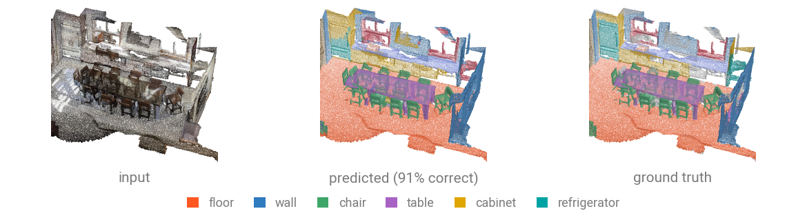
Download the sample_scene_labeled.ply (4.5 MB) to get started. This is a ScanNet room with RGB, mesh normals and NYU40 labels.
curl -LO https://github.com/arthurdjn/pytorch-pointcloud/raw/main/docs/assets/data/sample_scene_labeled.ply
The registered transform associated with the checkpoint (with return_info=True) provides the preprocessing used for evaluation and benchmarking on the associated dataset.
import numpy as np
import torch
from plyfile import PlyData

import torch_pointcloud as tp
import torch_pointcloud.transforms as T
from torch_pointcloud.datasets.scannet import SCANNET20_LABELS
from torch_pointcloud.utils.data import collate

ply = PlyData.read("sample_scene_labeled.ply")["vertex"]
pos = np.stack([ply["x"], ply["y"], ply["z"]], 1).astype("float32")
normal = np.stack([ply["nx"], ply["ny"], ply["nz"]], 1).astype("float32")
color = np.stack([ply["red"], ply["green"], ply["blue"]], 1).astype("float32")
segment = np.asarray(ply["segment"]).astype("int64")

sample = {
    "pos": torch.from_numpy(pos),
    "color": torch.from_numpy(color),
    "normal": torch.from_numpy(normal),  # the checkpoint reads color + normals
    "segment": torch.from_numpy(segment),
}
# the file's ids are NYU40, the benchmark's are not: a refrigerator is 24 in one and 15 in the other
sample = T.Relabel(keys="segment", labels=SCANNET20_LABELS)(sample)

# Load the pretrained model
model, info = tp.create_model(
    "spunet-v1m1.scannet20.pointcept",
    task="segmentation",
    pretrained=True,
    return_info=True,
)
model = model.cuda().eval()

# Get associated transform
transform = info["transform"]

# Apply the transform to the scene: it voxelizes in place and keeps the source cloud under `origin_*`
sample = transform(sample)
data = collate([sample])
print(f"Data keys: {data.keys()}")

with torch.no_grad():
    x = data["x"].cuda()
    pos_grid = data["pos_grid"].cuda()
    batch = data["batch"].cuda()
    inverse = data["inverse"].cuda()
    logits = model(x, pos_grid, batch)

# Get predictions at full resolution
preds = logits[inverse].argmax(dim=-1).cpu()
print(f"Logits shape: {tuple(logits.shape)}")
print(f"Predictions shape: {tuple(preds.shape)}")

# Data keys: dict_keys(['pos', 'color', 'normal', 'segment', 'x', 'origin_pos', 'origin_segment', 'pos_grid', 'inverse', 'batch'])
# Logits shape: (114118, 20)
# Predictions shape: (127410,)
Because the pipeline voxelizes the input scene, the model sees one point per 2 cm voxel.
The inverse tensor maps the predictions back to the original points, whose labels are kept under origin_segment.
Inputs and outputs
| Argument | Shape | Description |
|---|---|---|
x |
\((N, C)\) or None |
Per-point features usually color, normals, height. |
pos / pos_grid |
\((N, 3)\) | Coordinates (float) or integer voxel-grid coordinates (depends on the model) |
batch |
\((N,)\) | Index tensor associating each point to its point cloud |
| returns | \((N, \text{num\_classes})\) | Per-point logits |
Full-resolution predictions
Voxelization is part of the checkpoint, so raw logits are per voxel. Voxelize records the mapping under dst_inverse_key, and logits[inverse] scatters predictions back to every original point. Registered pipelines set it and keep the source cloud under origin_pos / origin_segment, so full-resolution scoring is logits[inverse] against origin_segment.
import torch
import torch_pointcloud.transforms as T

torch.manual_seed(0)

transform = T.Compose([
    T.Shift(keys="pos", method="min"),
    T.CopyItems(keys=["pos", "segment"], names=["origin_pos", "origin_segment"]),
    T.Voxelize(
        pos_key="pos",
        pos_reduce="grid",
        size=0.02,
        keys=["color", "segment"],
        dst_inverse_key="inverse",
    ),
])

sample = {
    "pos": torch.rand(20_000, 3) * 4.0,
    "color": torch.rand(20_000, 3) * 255,
    "segment": torch.randint(0, 20, (20_000,)),
}
sample = transform(sample)
print(f"Sample keys: {sample.keys()}")
print(f"Pos shape: {tuple(sample['pos'].shape)}")
print(f"Inverse shape: {tuple(sample['inverse'].shape)}")

# Sample keys: dict_keys(['pos', 'color', 'segment', 'origin_pos', 'origin_segment', 'inverse'])
# Pos shape: (19975, 3)
# Inverse shape: (20000,)
For rooms too large for one forward pass, an inferer tiles or sub-samples the scene and stitches the partial predictions back into one \((N, C)\) output.
Evaluate on a scene
You will find several utilities in torch_pointcloud.utils.metrics to score the predictions.
from torch_pointcloud.utils.metrics import confusion_matrix

cm = confusion_matrix(
    preds,
    data["segment"],
    num_classes=model.num_classes,
    ignore_index=-1,
)
intersection = cm.diag().float()
union = cm.sum(0).float() + cm.sum(1).float() - intersection
present = cm.sum(1) > 0

print(f"accuracy {cm.diag().sum() / cm.sum():.4f}")
print(f"mIoU     {(intersection[present] / union[present]).mean():.4f}")
# accuracy 0.9057
# mIoU     0.7440
Ignore the unlabeled points
ignore_index=-1 drops the unlabeled points from the confusion matrix.
Train from scratch
from tqdm.auto import tqdm
from torch.nn import functional as F
from torch.utils.data import DataLoader

import torch
import torch_pointcloud as tp
import torch_pointcloud.transforms as T
from torch_pointcloud.datasets import ShapeNetPart
from torch_pointcloud.utils.data import collate
from torch_pointcloud.config import DATA_DIR

device = "cuda"

# Setup the dataset and dataloader
train_dataset = ShapeNetPart(
    DATA_DIR,
    split="train",
    categories="Airplane",
    transform=T.Rescale(keys="pos"),
)
train_dataloader = DataLoader(
    train_dataset,
    batch_size=16,
    shuffle=True,
    num_workers=4,
    collate_fn=collate,
)

# Create the desired model and optimizer
model = tp.create_model(
    "pointnext-sm",
    task="segmentation",
    in_channels=0,
    num_classes=50,
).to(device)
optimizer = torch.optim.AdamW(
    model.parameters(),
    lr=1e-3,
    weight_decay=1e-4,
)

# Training loop
num_epochs = 1  # a demo pass, raise it to actually train

model.train()
for epoch in range(num_epochs):
    total_loss = 0.0
    pbar = tqdm(enumerate(train_dataloader), total=len(train_dataloader), desc=f"Epoch {epoch}")
    for i, data in pbar:
        pos = data["pos"].to(device)
        target = data["segment"].to(device)
        batch = data["batch"].to(device)

        optimizer.zero_grad()
        logits = model(None, pos, batch)
        logits = F.log_softmax(logits, dim=1)
        loss = F.nll_loss(logits, target)

        loss.backward()
        optimizer.step()
        total_loss += loss.item()
        if (i + 1) % 10 == 0:
            loss_step = loss.item()
            metrics = {"train/loss_step": f"{loss_step:.3f}"}
            pbar.set_postfix(metrics)

    loss_epoch = total_loss / len(train_dataloader)
    print(f"Loss epoch {epoch}: {loss_epoch:.3f}")


# Loading: 100%|██████████| 1958/1958 [00:00<00:00, 29210.61it/s]
# Epoch 0: 100%|██████████| 123/123 [00:02<00:00, 45.25it/s, train/loss_step=0.275]
# Loss epoch 0: 0.673
# Epoch 1: 100%|██████████| 123/123 [00:02<00:00, 45.30it/s, train/loss_step=0.220]
# Loss epoch 1: 0.244
# Epoch 2: 100%|██████████| 123/123 [00:02<00:00, 45.30it/s, train/loss_step=0.220]
# Loss epoch 2: 0.228
# Epoch 3: 100%|██████████| 123/123 [00:02<00:00, 44.70it/s, train/loss_step=0.223]
# Loss epoch 3: 0.221
# Epoch 4: 100%|██████████| 123/123 [00:02<00:00, 45.24it/s, train/loss_step=0.190]
# Loss epoch 4: 0.215
# Epoch 5: 100%|██████████| 123/123 [00:02<00:00, 45.52it/s, train/loss_step=0.231]
# Loss epoch 5: 0.211
# Epoch 6: 100%|██████████| 123/123 [00:02<00:00, 45.86it/s, train/loss_step=0.170]
# Loss epoch 6: 0.208
# Epoch 7: 100%|██████████| 123/123 [00:02<00:00, 45.59it/s, train/loss_step=0.168]
# Loss epoch 7: 0.205
# Epoch 8: 100%|██████████| 123/123 [00:02<00:00, 45.94it/s, train/loss_step=0.195]
# Loss epoch 8: 0.199
# Epoch 9: 100%|██████████| 123/123 [00:02<00:00, 44.63it/s, train/loss_step=0.161]
# Loss epoch 9: 0.198
Outdoor LiDAR
Similarly to the above example, you can run a LiDAR segmentation model on a sample scan. The spvcnn-119gmacs.semantickitti.mit-han-lab model
takes intensity rather than color and voxelizes at 5 cm.
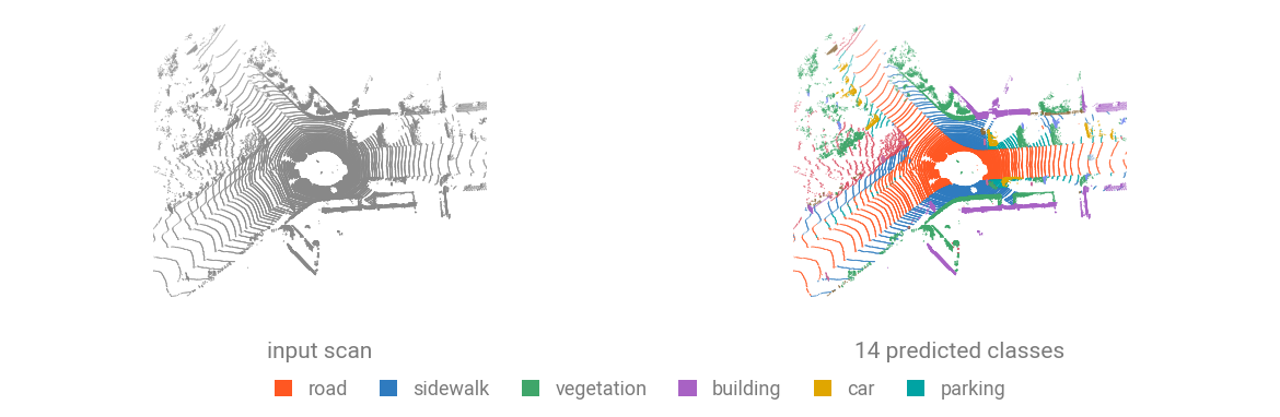
Download the sample_lidar_a.ply (2.3 MB) to get started. This is a SemanticKITTI scan with intensity and ground truth labels.