Train a model
Open in Colab · Download notebook
This notebook will guide you on how to train a model using torch-pointcloud and raw PyTorch and at the end how to wrap it in PyTorch Lightning.
Models from torch-pointcloud are plain nn.Modules that take packed tensors, so there is no framework to learn: a standard PyTorch training loop works as-is.
Setup
import torch

import torch_pointcloud as tp
import torch_pointcloud.transforms as T
from torch_pointcloud.utils.data import PointCloudDataLoader

DEVICE = "cuda" if torch.cuda.is_available() else "cpu"
NUM_POINTS = 1024
BATCH_SIZE = 32
EPOCHS = 5

torch.manual_seed(0)
DEVICE
Data
ModelNet40 ships CAD meshes, so the transform samples points on the faces and normalizes the result. The train transform adds augmentation on top whereas the validation transform stays deterministic so validation numbers are comparable across epochs.
from torch_pointcloud.datasets import ModelNet40

val_transform = T.Compose([
    T.Rescale(keys="pos", method="centroid"),
    T.RandomSampleFaceVertices(keys="pos", face_key="face", num_samples=NUM_POINTS),
    T.KeepItems(keys=["pos", "normal", "label"]),
])
train_transform = T.Compose([
    val_transform,
    T.RandomScale(keys="pos", scale_range=(0.8, 1.2)),
    T.RandomJitter(keys="pos", sigma=0.01, clip=0.05),
])

train_dataset = ModelNet40(root="data", train=True, transform=train_transform, download=True)
val_dataset = ModelNet40(root="data", train=False, transform=val_transform, download=True)
print(f"Train dataset: {len(train_dataset):,} | Val dataset: {len(val_dataset):,}")
Packed batches
Point clouds have different point counts, so batches are packed: every cloud is concatenated along axis 0 and a batch index tags each point with the cloud it came from. Here we use the torch_pointcloud.utils.data.PointCloudDataLoader dataloader, which is a DataLoader with a custom collate function used to pack input data.
train_dataloader = PointCloudDataLoader(train_dataset, batch_size=BATCH_SIZE, shuffle=True, drop_last=True)
val_dataloader = PointCloudDataLoader(val_dataset, batch_size=BATCH_SIZE, shuffle=False)

data = next(iter(train_dataloader))
{k: tuple(v.shape) for k, v in data.items() if torch.is_tensor(v)}
# {'pos': (32768, 3), 'normal': (32768, 3), 'label': (32,), 'batch': (32768,)}
pos is \((N, 3)\) with \(N = 32 \times 1024\) points from 32 clouds, batch is \((N,)\), and label is \((B,)\): one class per cloud.
Model
Next we use the create_model to instantiate a model with a registered architecture. pretrained=False (the default) gives random weights. You can of course instantiate your model of interest from the class itself, it is a standard nn.Module and recommended for training a model from scratch as it makes the instantiation explicit (no **kwargs forwarded).
from torch_pointcloud.models import PointNet2Classification


model = PointNet2Classification(
        in_channels=0,
        num_classes=40,
        sa_channels=[[64, 64, 128], [128, 128, 256]],
        aggr_channels=[256, 512, 1024],
        aggr_use_pos=True,
        head_channels=[512, 256],
        ratios=[0.5, 0.25],
        radii=[0.2, 0.4],
        num_neighbors=[32, 64],
        use_pos=True,
        normalize_pos=False,
        bias=True,
        dropout=0.4,
).to(DEVICE)
print(f"{sum(p.numel() for p in model.parameters()) / 1e6:.2f}M parameters")
print("signature: model(x, pos, batch)")
print("in_channels:", model.in_channels, "| num_classes:", model.num_classes)
Classification models take (x, pos, batch) and return \((B, C)\) logits. This configuration has in_channels = 0, meaning it learns from geometry alone, so x is None. A model configured with in_channels = 6 would instead receive 6 input channels, for example x = torch.cat([pos, normal], dim=1).
Optimizer, scheduler, loss
We define in the cell below the optimizer, scheduler and loss function.
optimizer = torch.optim.AdamW(model.parameters(), lr=1e-3, weight_decay=1e-4)
scheduler = torch.optim.lr_scheduler.CosineAnnealingLR(optimizer, T_max=EPOCHS * len(train_dataloader))
criterion = torch.nn.CrossEntropyLoss()
The training loop
The training loop is plain PyTorch. To train a model, you can use the following code:
from tqdm.auto import tqdm


def train_one_epoch(model, dataloader, optimizer, scheduler, criterion, device):
    model.train()
    total_loss, total_correct, total_seen = 0.0, 0, 0

    for data in tqdm(dataloader, desc="Training"):
        pos = data["pos"].to(device)
        batch = data["batch"].to(device)
        target = data["label"].to(device)

        optimizer.zero_grad()
        logits = model(None, pos, batch)
        loss = criterion(logits, target)
        loss.backward()
        optimizer.step()
        scheduler.step()

        total_loss += loss.item() * target.numel()
        total_correct += int(logits.argmax(dim=1).eq(target).sum())
        total_seen += target.numel()

    return {"loss": total_loss / total_seen, "acc": total_correct / total_seen}
@torch.no_grad()
def evaluate(model, dataloader, criterion, device):
    model.eval()
    total_loss, total_correct, total_seen = 0.0, 0, 0

    for data in tqdm(dataloader, desc="Evaluating"):
        pos = data["pos"].to(device)
        batch = data["batch"].to(device)
        target = data["label"].to(device)

        logits = model(None, pos, batch)
        total_loss += criterion(logits, target).item() * target.numel()
        total_correct += int(logits.argmax(dim=1).eq(target).sum())
        total_seen += target.numel()

    return {"loss": total_loss / total_seen, "acc": total_correct / total_seen}
history = []

for epoch in range(EPOCHS):
    train_metrics = train_one_epoch(model, train_dataloader, optimizer, scheduler, criterion, DEVICE)
    val_metrics = evaluate(model, val_dataloader, criterion, DEVICE)
    history.append({"epoch": epoch + 1, "train": train_metrics, "val": val_metrics})
    print(
        f"epoch {epoch + 1}/{EPOCHS}"
        f" | train loss {train_metrics['loss']:.3f} acc {train_metrics['acc']:.3f}"
        f" | val loss {val_metrics['loss']:.3f} acc {val_metrics['acc']:.3f}"
    )
import matplotlib.pyplot as plt

epochs = [entry["epoch"] for entry in history]

_, axes = plt.subplots(1, 2, figsize=(10.0, 4.0))
for ax, key, name in zip(axes, ("loss", "acc"), ("loss", "accuracy")):
    ax.plot(epochs, [entry["train"][key] for entry in history], marker="o", label="train")
    ax.plot(epochs, [entry["val"][key] for entry in history], marker="o", label="val")
    ax.set(xlabel="epoch", ylabel=name)
    ax.set_xticks(epochs)
    ax.legend(frameon=False, fontsize=9)
    ax.spines["top"].set_visible(False)
    ax.spines["right"].set_visible(False)
plt.show()
Where the errors are
Overall accuracy says nothing about which of the 40 classes go wrong. A confusion matrix does: reload the run's best checkpoint, replay the test split, and count how often each true class lands on each predicted one.
return_info=True hands back the evaluation transform the checkpoint was validated with, so the replay preprocesses its input the way the run did.
import matplotlib.pyplot as plt
from torchmetrics.classification import MulticlassConfusionMatrix

metric = MulticlassConfusionMatrix(num_classes=40)

model.eval()
with torch.no_grad():
    for data in tqdm(val_dataloader, desc="Confusion matrix"):
        logits = model(None, data["pos"].to(DEVICE), data["batch"].to(DEVICE))
        metric.update(logits.argmax(dim=1).cpu(), data["label"])

confusion = metric.compute()
rows = confusion / confusion.sum(dim=1, keepdim=True).clamp(min=1)

_, ax = plt.subplots(figsize=(11.0, 10.0))
image = ax.imshow(rows, cmap="Oranges", vmin=0.0, vmax=1.0)
ax.set_xticks(range(40), val_dataset.classes, rotation=90, fontsize=8)
ax.set_yticks(range(40), val_dataset.classes, fontsize=8)
ax.set(xlabel="predicted", ylabel="true")
plt.colorbar(image, ax=ax, label="fraction of a true class")
plt.show()
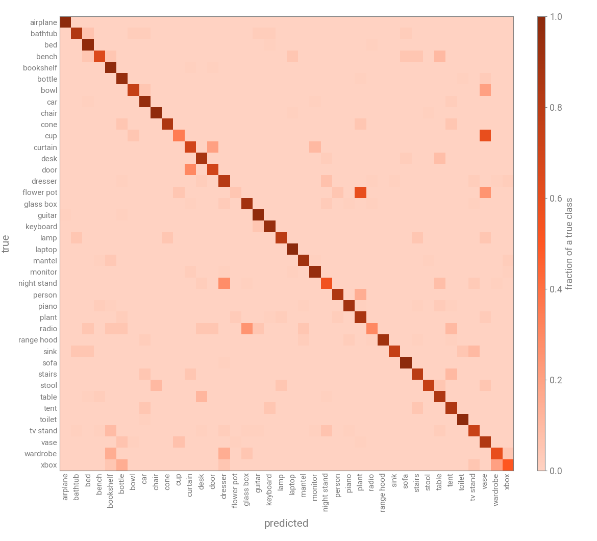
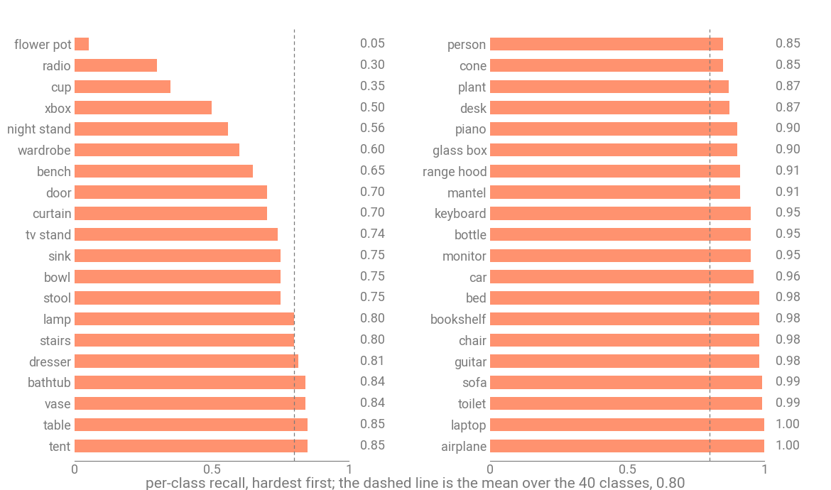
Every row is one true class and sums to 1, so the diagonal is that class's recall and the bright cells beside it are where its meshes went instead. The bright off-diagonal cells fall on the near-duplicate categories: ModelNet40 keeps plant and flower_pot, desk and table, dresser and night_stand as separate classes, and 1024 sampled points do not always tell them apart.
recall = confusion.diag() / confusion.sum(dim=1).clamp(min=1)
ranked = sorted(zip(val_dataset.classes, recall.tolist()), key=lambda entry: entry[1])

print(f"overall {confusion.diag().sum() / confusion.sum():.3f} | mean per class {recall.mean():.3f}")
for name, value in ranked[:5]:
    print(f"{name:<12} {value:.2f}")

_, ax = plt.subplots(figsize=(7.0, 9.0))
ax.barh([name for name, _ in ranked], [value for _, value in ranked], height=0.7)
ax.axvline(recall.mean(), linewidth=0.9, linestyle="--")
ax.invert_yaxis()
ax.set(xlabel="recall", xlim=(0, 1))
plt.show()
Save and reload
Weights are a plain state_dict. Reload them into a fresh architecture built by the same create_model call.
torch.save(model.state_dict(), "pointnet2_modelnet40.pt")

reloaded = tp.create_model("pointnet2-ssg.modelnet40.xu-yan", task="classification")
reloaded.load_state_dict(torch.load("pointnet2_modelnet40.pt", weights_only=True))
reloaded.eval();
The same run with Lightning
Everything above is the loop Lightning would otherwise write for you. The lightning extra (pip install "torch-pointcloud[lightning]") provides two wrappers:
PointCloudDataModulebuilds the packed loaders from the datasets.LitClassificationModeltakes the same model namecreate_modeldoes, and owns the loop, the logging and the checkpointing.
from functools import partial

import lightning.pytorch as L
from torchmetrics.classification import MulticlassAccuracy

from torch_pointcloud.lightning import LitClassificationModel, MetricCallback, PointCloudDataModule

datamodule = PointCloudDataModule(
    train_dataset=train_dataset,
    val_dataset=val_dataset,
    batch_size=BATCH_SIZE,
    num_workers=0,
)
lit = LitClassificationModel(
    "pointnet2-ssg.modelnet40.xu-yan",
    optimizer=partial(torch.optim.AdamW, lr=1e-3, weight_decay=1e-4),
    scheduler=partial(torch.optim.lr_scheduler.CosineAnnealingLR, T_max=200),
    target_key="label",
)

trainer = L.Trainer(
    max_epochs=EPOCHS,
    accelerator="auto",
    logger=False,
    enable_checkpointing=False,
    callbacks=[MetricCallback(MulticlassAccuracy(num_classes=40), name="acc")],
)
trainer.fit(lit, datamodule=datamodule)
trainer.validate replays the validation loop on its own, printing the same val/loss and val/acc the plain loop computed by hand.