Detect objects in driving LiDAR¶

This notebook will guide you on how to detect objects from LiDAR data using a pretrained model.

Setup¶

# On Colab: !pip install "torch-pointcloud"
# On Colab: !pip install torch-scatter torch-cluster -f https://data.pyg.org/whl/torch-2.10.0+cu128.html
import numpy as np
import torch

import torch_pointcloud as tp
import torch_pointcloud.transforms as T

torch.manual_seed(0)
device = "cuda" if torch.cuda.is_available() else "cpu"
print("torch-pointcloud", tp.__version__, "| device:", device)

Helpers¶

Let's define some helpers to visualize the data.

import matplotlib.pyplot as plt
from mpl_toolkits.mplot3d.art3d import Line3DCollection

from torch_pointcloud.utils.box3d import box_corners

PLAN, SIDE = (88, -90), (26, -84)  # elevation and azimuth: straight down, and from the driver's side
BOX_EDGES = ((0, 1), (1, 2), (2, 3), (3, 0), (4, 5), (5, 6), (6, 7), (7, 4), (0, 4), (1, 5), (2, 6), (3, 7))


def show_cloud(pos, color=None, *, ax=None, title=None, size=1.2, view=SIDE, cmap="viridis"):
    """Scatter a sweep. `pos` is (N, 3); `color` is a per-point scalar, a matplotlib color, or None."""
    if ax is None:
        ax = plt.figure(figsize=(7, 4)).add_subplot(projection="3d")
    p = pos.cpu().numpy()
    c = color.cpu().numpy() if torch.is_tensor(color) else color
    kw = {"cmap": cmap} if c is not None and np.ndim(c) == 1 else {}
    ax.scatter(p[:, 0], p[:, 1], p[:, 2], c=c, s=size, depthshade=False, linewidths=0, **kw)
    ax.view_init(elev=view[0], azim=view[1])
    span = p.max(0) - p.min(0)
    ax.set_box_aspect(np.maximum(span, 0.02 * span.max()))  # a sheet of pillars is flat in z, which has no aspect
    ax.set_axis_off()
    if title:
        ax.set_title(title, fontsize=10)
    return ax


def show_boxes(ax, boxes, colors, linestyle="-"):
    """Draw (K, 7) oriented boxes on a 3D axes as one wireframe per row, heading included."""
    for corners, color in zip(box_corners(boxes).cpu().numpy(), colors):
        segments = [(corners[a], corners[b]) for a, b in BOX_EDGES]
        ax.add_collection3d(Line3DCollection(segments, colors=color, linewidths=1.2, linestyles=linestyle))

Data¶

We will read one frame of the KITTI 3D object benchmark and detect objects on the road. The dataset has no automatic download: get it from its download page and extract it under data/KITTI/raw/.

from torch_pointcloud.datasets import KITTI

dataset = KITTI(root="data", train=True, fov=True)

data = dataset[211]

pos = data["pos"]
print("points:", len(pos))
for axis, name in enumerate(("x forward", "y left  ", "z up    ")):
    print(f"  {name}: {float(pos[:, axis].min()):6.1f} to {float(pos[:, axis].max()):5.1f} m")

horizontal = pos[:, :2].norm(dim=1)
print("max horizontal range:", round(float(horizontal.max()), 1), "m")
print("points within 20 m:", int((horizontal < 20).sum()), "| beyond 40 m:", int((horizontal >= 40).sum()))
print("intensity:", round(float(data["intensity"].min()), 2), "to", round(float(data["intensity"].max()), 2), "| mean", round(float(data["intensity"].mean()), 2))
print("ground plane (1st percentile of z):", round(float(pos[:, 2].quantile(0.01)), 2), "m")

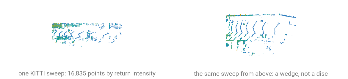
16 835 points, out to 80 m, with the sensor at the origin. Every driving detector in the library assumes these conventions:

\(+x\) is forward, \(+y\) is left, \(+z\) is up, with the origin at the LiDAR. Nothing is centered or normalized: a detector defines its voxel grid in meters in this frame, so recentering the cloud would move the whole scene out of range.
The ground is a plane at \(z \approx -1.75\) m, the sensor's mount height. That is why the anchor boxes below sit at fixed heights instead of being regressed from scratch.
The sweep is cropped to the front camera's field of view. KITTI only annotates what the left color camera sees, so the standard protocol (KITTI(..., fov=True)) drops the rest of the 360-degree sweep. That is the wedge you see from above.

A box is 7 numbers, \((c_x, c_y, c_z, d_x, d_y, d_z, \theta)\): center, full extents, and a heading counter-clockwise about \(+z\) from \(+x\). The center is the box center, not the ground contact point.

intensity = data["intensity"].squeeze(1)

fig = plt.figure(figsize=(12, 4))
show_cloud(pos, intensity, ax=fig.add_subplot(121, projection="3d"), title=f"one KITTI sweep: {len(pos):,} points by return intensity")
show_cloud(pos, intensity, ax=fig.add_subplot(122, projection="3d"), view=PLAN,  title="the same sweep from above");

KITTI sweep colored by intensity

from torch_pointcloud.datasets.kitti import KITTI_CLASSES

for box, label in zip(data["box"], data["label"]):
    distance = float(box[:2].norm())
    print(f"  {KITTI_CLASSES[int(label)]:8s} at {distance:5.1f} m"
          f"  size ({float(box[3]):.2f}, {float(box[4]):.2f}, {float(box[5]):.2f}) m"
          f"  heading {float(box[6]):+.2f} rad"
          f"  bottom z {float(box[2] - box[5] / 2):+.2f} m")

Five cars and three cyclists, from 5.4 m to 45.3 m out. Two things to notice: every box bottom lands within \(40\) cm of the \(-1.75\) m ground plane, which is the regularity anchor-based detectors exploit. And every heading is within \(0.1\) rad of \(0\) or \(\pi\): this is a straight road and everything on it is aligned with the lane.

What a pillar encoder needs¶

PointPillars quantizes the data into a 2D grid of vertical pillars (hence the name), stacks the points that fall in each one, and runs a 2D CNN over the resulting bird's-eye feature map. It is configured by:

parameter	value	why
`point_cloud_range`	\((0, -39.68, -3) \to (69.12, 39.68, 1)\) m	forward half only (KITTI annotates the camera view), 4 m of height, sized so the grid divides evenly
`voxel_size`	\((0.16, 0.16, 4.0)\) m	16 cm in the ground plane; the full height in one cell, which is what makes a pillar rather than a voxel
`max_num_points`	32	points per pillar the encoder reads; the stack is padded below it and truncated above

transform = T.Compose([
    T.Cat(keys=["intensity"], dst_key="x", dim=1),
    T.HardVoxelize(
        pos_key="pos",
        feat_key="x",
        voxel_size=(0.16, 0.16, 4.0),
        point_cloud_range=(0.0, -39.68, -3.0, 69.12, 39.68, 1.0),
        max_num_points=32,
        max_num_voxels=40000,
    ),
])

sample = transform({"pos": pos.clone(), "intensity": data["intensity"].clone()})
print({k: tuple(v.shape) for k, v in sample.items() if torch.is_tensor(v)})

cells = round(69.12 / 0.16) * round(79.36 / 0.16)
counts = sample["voxel_num_points"]
print("occupied pillars:", len(counts), f"of {cells} grid cells ({100 * len(counts) / cells:.2f}%)")
print("points kept:", int(counts.sum()), "of", len(pos))
print("points per pillar: mean", round(float(counts.float().mean()), 1), "| full (32):", int((counts == 32).sum()))

voxel is a \((4055, 32, 4)\) tensor, i.e. 4055 occupied pillars, up to 32 points each and four channels per point \((x, y, z, \text{intensity})\). The pos_voxel tensor is the integer grid index \((z, y, x)\) of each pillar and voxel_num_points says how many of the 32 slots are real.

voxel_size = torch.tensor([0.16, 0.16, 4.0])
origin = torch.tensor([0.0, -39.68, -3.0])
centers = sample["pos_voxel"].flip(1).float() * voxel_size + origin + voxel_size / 2

show_cloud(centers, size=0.6, view=PLAN, title=f"{len(centers):,} occupied pillars of 0.16 m");

pos_voxel is stored as \((z, y, x)\), so it is flipped before it is scaled back into meters. Every pillar comes out at \(z = -1\) m, the middle of the 4 m range, because the grid has exactly one cell in \(z\): that is what makes a pillar rather than a voxel, and it is why the plot above is a sheet rather than a volume.

Seen from above the 16 cm lattice resolves in the near field: the laser rings of the sweep become rows of cells, and the gaps between rings become empty ones.

Decoding the head¶

A detection head emits a dense field of proposals: one per anchor, per grid cell and unfiltered. model.decode(out) unpacks that into a flat Detection3D. Thresholding and NMS belong to the evaluation protocol, so you choose the post-processing and can swap it out.

Detection3D is a plain dictionary of packed tensors containing:

key	shape	meaning
`boxes`	\((K, 7)\)	\((c_x, c_y, c_z, d_x, d_y, d_z, \theta)\), full extents
`labels`	\((K,)\)	class index per box
`scores`	\((K,)\)	confidence per box
`batch`	\((K,)\)	which scene of the batch each box belongs to

Boxes3D is the same without scores, and is what ground truth is carried in.

Run a pretrained checkpoint¶

We will use create_model to instantiate the pretrained model pointpillars.kitti.openpcdet, a PointPillars trained on the KITTI 3-class split.

model, info = tp.create_model(
    "pointpillars.kitti.openpcdet",
    task="detection",
    pretrained=True,
    return_info=True,
)
model = model.to(device).eval()

print("classes:", info["weights"]["classes"])
print(info["transform"])

return_info=True also returns the checkpoint's registry entry, including the transform it was evaluated with.

collate packs a list of samples into a batch and will create the batch tensor index. Pillars are ragged across scenes, so pos_voxel is concatenated rather than stacked and the dataloader synthesizes a batch_pos_voxel index naming the scene each pillar came from.

from torch_pointcloud.utils.data import collate

batch = collate(
    [info["transform"]({"pos": pos.clone(), "intensity": data["intensity"].clone()})],
    cat_keys=["pos_voxel"],
)

with torch.no_grad():
    out = model(
        batch["voxel"].to(device),
        batch["pos_voxel"].to(device),
        batch["voxel_num_points"].to(device),
        batch["batch_pos_voxel"].to(device),
    )

print("head output:", {k: tuple(v.shape) for k, v in out.items()})
print("anchors:", tuple(model.head.anchors.shape))
# head output: {'cls': (1, 248, 216, 18), 'box': (1, 248, 216, 42), 'dir_cls': (1, 248, 216, 12), 'batch_cls': (1, 321408, 3), 'batch_box': (1, 321408, 7)}
# anchors: (321408, 7)

The head format is specific to the model. Here it contains cls, box and dir_cls which are the three \(1 \times 1\) convolutions of the anchor head, still shaped as a \(248 \times 216\) bird's-eye feature map. There are 6 anchors per cell (3 classes, each at \(0\) and \(\pi/2\)), so the channel counts are \(6 \times 3 = 18\) class logits, \(6 \times 7 = 42\) box residuals and \(6 \times 2 = 12\) direction-bin logits.

batch_cls and batch_box are those same predictions flattened and already decoded against the anchors: \(248 \times 216 \times 6 = 321\,408\) absolute boxes in meters, and one class logit vector per box.

To actually decode this format into Detection3D, we will use the decode method:

detections = model.decode(out)
print({k: tuple(v.shape) for k, v in detections.items()})
print("score range:", round(float(detections["scores"].min()), 4), "to", round(float(detections["scores"].max()), 4))

above = detections["scores"] > 0.1
boxes, scores = detections["boxes"][above], detections["scores"][above]
labels, index = detections["labels"][above], detections["batch"][above]
print("above score 0.10:", int(above.sum()))

That applies no filtering. We apply NMS by hand to remove duplicate boxes: where several boxes overlap, it keeps the highest scoring one.

from torch_pointcloud.utils.box3d import nms3d

index = nms3d(boxes, scores, 0.01, batch=index, rotated=True)
boxes, scores, labels = boxes[index].cpu(), scores[index].cpu(), labels[index].cpu()
print("after 3D NMS:", len(boxes))

final = scores > 0.5
print("above score 0.50:", int(final.sum()))

CLASS_COLOR = ["tab:orange", "tab:blue", "tab:green"]  # Car, Pedestrian, Cyclist

classes = info["weights"]["classes"]
near = pos[pos[:, 0] < 50]  # the far quarter of the sweep holds no annotated object
scored = detections["boxes"][above].cpu()
scored_labels = detections["labels"][above].cpu()

stages = [(f"{len(scored)} boxes above score 0.10", scored, scored_labels),
          (f"{len(boxes)} boxes after 3D NMS", boxes, labels)]

fig = plt.figure(figsize=(12, 5))
for index, (title, stage_boxes, stage_labels) in enumerate(stages):
    ax = fig.add_subplot(1, 2, index + 1, projection="3d")
    ax = show_cloud(near, "0.6", ax=ax, title=title, size=0.5, view=PLAN)
    show_boxes(ax, stage_boxes, [CLASS_COLOR[int(label)] for label in stage_labels])

Boxes before and after NMS

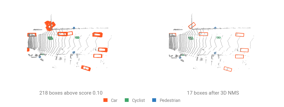
The NMS call above cut 218 boxes down to 17. Filtering on a score above \(0.5\) reduces that to 8:

for box, score, label in zip(boxes[final], scores[final], labels[final]):
    print(f"  {classes[int(label)]:8s} {float(score):.2f}"
          f"  center ({float(box[0]):5.1f}, {float(box[1]):5.1f}, {float(box[2]):+.2f})"
          f"  size ({float(box[3]):.2f}, {float(box[4]):.2f}, {float(box[5]):.2f})"
          f"  heading {float(box[6]):+.2f}")

Here eight detections are left: five cars and three cyclists, scored 0.74 to 0.94.

fig = plt.figure(figsize=(12, 5))
shown = f"{int(final.sum())} predicted boxes over the {len(data['box'])} annotations"
for index, (view, angle) in enumerate(((PLAN, "from above"), (SIDE, "from the driver's side"))):
    ax = fig.add_subplot(1, 2, index + 1, projection="3d")
    ax = show_cloud(near, "0.6", ax=ax, size=0.5, view=view, title=f"{shown}, {angle}")
    show_boxes(ax, data["box"], ["0.35"] * len(data["box"]), linestyle="--")
    show_boxes(ax, boxes[final], [CLASS_COLOR[int(label)] for label in labels[final]])

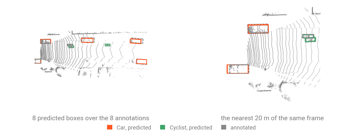
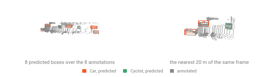
Predictions versus annotations, top view

Predictions versus annotations, side view

Eight predictions over eight ground truth annotations. The predictions are drawn solid and class-colored, the annotations dashed and gray.

from torch_pointcloud.utils.box3d import boxes_iou3d, count_points_in_boxes

overlap = boxes_iou3d(boxes[final], data["box"])
returns = count_points_in_boxes(pos, data["box"])
for row, (score, label) in enumerate(zip(scores[final], labels[final])):
    column = int(overlap[row].argmax())
    print(f"  {classes[int(label)]:8s} {float(score):.2f}"
          f"  ->  {KITTI_CLASSES[int(data['label'][column])]:8s}"
          f"  at {float(data['box'][column, :2].norm()):5.1f} m"
          f"  3D IoU {float(overlap[row, column]):.2f}"
          f"  on {int(returns[column]):4d} points")
print("ground-truth boxes recovered at IoU 0.5:", int((overlap.max(dim=0).values > 0.5).sum()), "of", len(data["box"]))

All eight objects are found, with 3D IoU from 0.54 to 0.84.